Real-Time Sentiment Analysis with Kafka & Spark Streaming
In this post, we will explore different aspects of Natural Language Processing, through a sentiment analysis of tweets retrieved from the social network Twitter. We will work with Apache Spark to test different techniques and determine which ones are the most interesting. Throughout this assignment, we will put ourselves in a Big Data context, where we will be dealing with large volumes of data, proving once again the usefulness of Spark and its Python implementation, PySpark.
The second part of this project was to deploy the best model in an ETL process using Kafka and Spark Streaming for real-time analysis on a topic of our choice.
It was made in collaboration with Thomas Sirvent for a course on Machine Learning for Big Data at UQAC.
Dataset : Sentiment140
Sentiment140 [1] is a well-known dataset when it comes to analyzing the sentiment of tweets. It was created by Alec Go, Richa Bhayani and Lei Huang, who were computer science students at Stanford University. Since then, it has been used in a number of scientific papers and thus serves as a benchmark for comparing the accuracy of models.
The dataset includes 1 600 000 tweets in the following format:
- the polarity of the tweet (0 = negative, 2 = neutral, 4 = positive)
- the ID of the tweet
- the date of the tweet
- the query used
- the user who tweeted
- the text of the tweet
For the polarity calculation, rather than going through a lengthy human annotation process, they assumed that all tweets containing positive emoticons, such as :), are positive, and tweets containing negative emoticons, such as :(, are negative.
Features Extraction
In this section, we will present all of the features that we attempted to extract from the input data. Not all of them have been retained for the final model (see Evaluation below).
HashingTF vs CountVectorizer
Both HashingTF and CountVectorizer can be used to generate term frequency vectors. However, they differ in a few ways.
HashingTF converts documents into vectors of fixed size. The default feature size is 262 144. The terms are mapped into indices using a hash function. The hash function used is MurmurHash 3. The frequencies of the terms are calculated with respect to the mapped indices.
While CountVectorizer will first generate a vocabulary. This step will be followed by the fitting of the CountVectorizer model. During the fitting process, CountVectorizer will select the top VocabSize words ranked by term frequency. The model will produce a vector that can be used later.
In sum, HashingTF is less expensive, as it uses a hash function, but is irreversible and can cause collisions, while CountVectorizer is deterministic and reversible, but is much more expensive.
IDF
The vectors then go through the IDF function (Inverse Document Frequency) which will, according to the formula below, filter the terms that do not appear a minimum number of times.
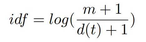
Where m is the total number of documents, and d(t) is the number of documents that contain the term t.
N-Gram
To give more context to the pattern, we use bag of words or N-gram to group words into groups of 2, 3, 4 or more consecutive words. These are called bi-grams, trigrams and quadrigrams.
ChiSqSelector
At the end of the pipeline, we also experimented with selecting the best features using Spark’s ChiSqSelector function. Indeed, with the creation of the N-grams presented above, the number of features started to become much too large. So we decided to select the best ones in order to reduce the search space.
Evaluation
The models were evaluated locally for simplicity. Below in Table 1 is the comparison of the models tested. This comparison is based on the accuracy metric and evaluates the models in each of the imagined feature scenarios.
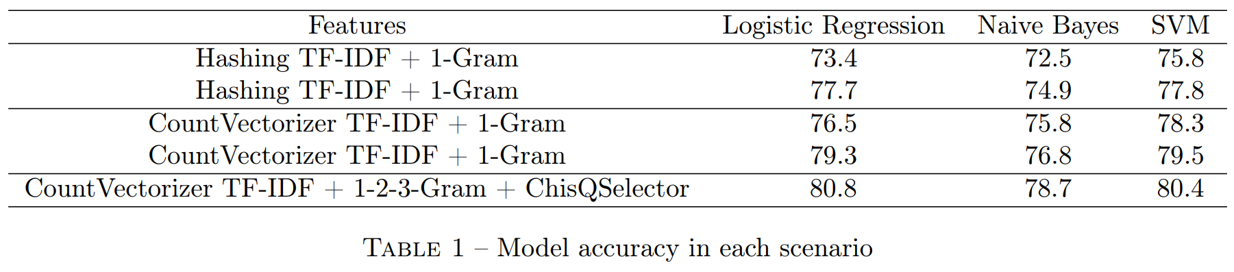
As our experimental results show, it is the Logistic Regression model that is the most adapted to our data with an accuracy of 80.8% in the last scenario. Also, we experimented in each scenario, different combinations of hyperparameters. When we explained the difference between HashingTF and CountVectorizer above, we pointed out that the former can cause collisions. It is this difference that we believe explains the differences in accuracy that can be noted between the scenarios with HashingTF versus CountVectorizer, which is admittedly longer, but does not lose any information.
In the last scenario, here are the parameters of our hyperparameter extraction functions in more detail.
- CountVectorizer : vocabulary size = 2^14
- IDF: Minimum Frequency = 5
- N-gram : 1-Gram, 2-Gram, 3-Gram
- ChiSqSelector : Top 2^14 features that is 16 384
That is a total of 49 152 features before the selection and 16 384 after the ChiSqSelector passage in the pipeline.
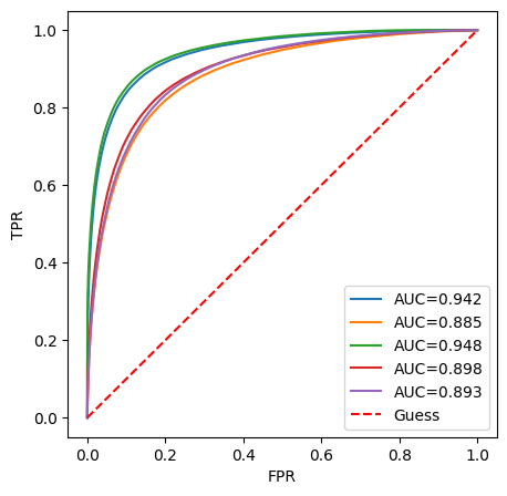
In more detail, you will find below two visualizations of the results of the logistic regression model.
First, we have displayed the ROC curves for each scenario with the logistic regression model. You can find on the abscissa the false positive rate and on the ordinate the true positive rate. The models shown in the legend are in the same order as in the table. We can notice that it is not the model with the highest precision that obtains the highest AUC value.
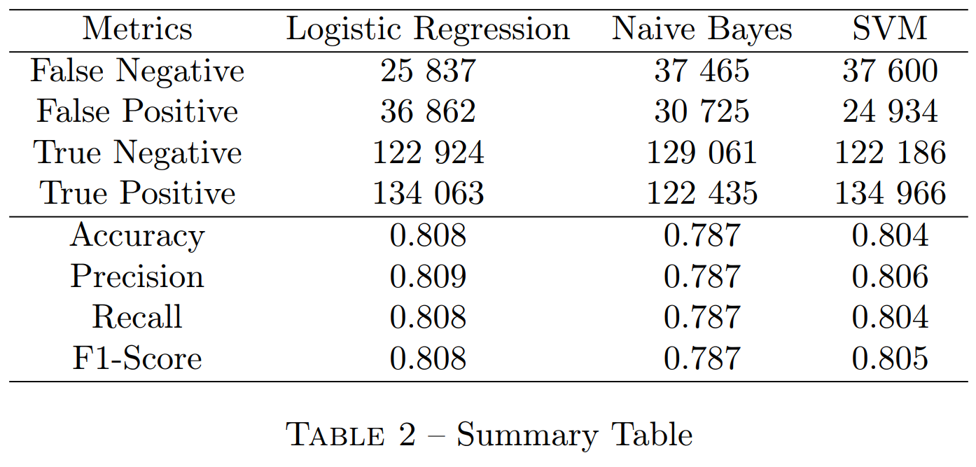
In more detail, if we focus on the logistic regression model in the last scenario, we can visualize its confusion matrix.
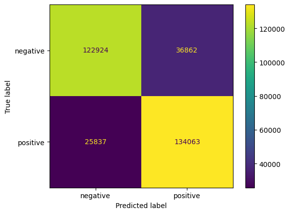
From this confusion matrix, we can see that this model is rather optimistic about the emotion of a tweet. Indeed, it labeled 36,862 tweets as positive when they were negative against only 25,837 positive tweets predicted as negative on the other side of the matrix.
Since we know that good accuracy does not necessarily imply that the model is the best for all metrics, you will find in Table 2 the summary of all metrics for all models in the last feature scenario.
Scaling-up
Google Cloud
To illustrate the scaling, we used the Google Cloud platform. Indeed, this one offers a 90-day free trial and a 300$ credit, in order to experiment with their resources the execution of Python scripts, Jupyter notebooks, or R. The Spark configuration is already done, so you can set up an environment very quickly.
Once the free trial has started, we need to start by creating an online storage space, called Bucket. Once initialized, we have to put all the datasets and scripts we are going to use in it. When we want to use these resources, we will have to use a relative path specific to the bucket, starting with “gs://”.
When we created the cluster, we opted for the following configuration:
- Master node
- 4 virtual processors, 16 GB of RAM
- Worker nodes
- 6 * 4 virtual processors, 15 GB RAM
Once the resources have been allocated, we obtain the set of nodes we had chosen.
Concretely, this platform will allow us to test large datasets without monopolizing our local machines. Once the cluster is up and running, all we have to do is go to the Interface Webs section and go to Jupyter or JupyterLab to start coding our processes. In our case, we often had problems maintaining a connection with Jupyter, so we focused on the Send Job feature, where we could point to a Python script present in our Bucket and make it work in a similar way to the spark submit command.
Results
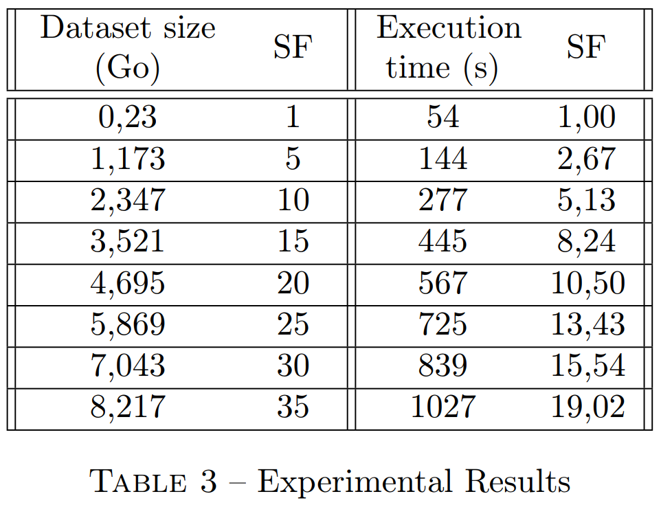
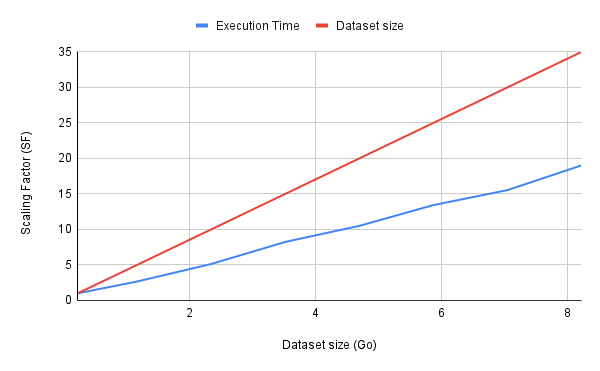
We defined a scaling factor of 1 per 233 MB for the size of the dataset and 1 per 54 seconds for the execution time. We then duplicated the dataset until we reached a scaling factor of 35, i.e. 8.2GB. You will find below the table summarizing the values as well as a graph showing the success of the scaling.
ETL : Deploying the best model
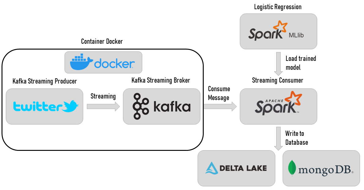
You can find more details about the implementation of this ETL process on my blog.
Used Software and Libraries
- Programming languages: Python
- Libraries: PySpark, Apache Kafka
- Source control: GitHub
- Other tools: Google Cloud, Jupyter Notebook, DataSpell
References
[1] Alec Go, Richa Bhayani et Lei Huang. « Twitter sentiment classification using distant supervision ». In : CS224N project report, Stanford 1.12 (2009), p. 2009.